Importing a parameter from a CSV file

After creating a parameter from the “Variable” drop-down in the “Insert” menu, right-clicking the parameter and selecting the option to “Import CSV”, will open a dialogue box that allows you to select a CSV file. Upon selecting the file, a dialog is opened, allowing you to specify assorted encoding parameters.

An alternative is to click on the ImportData icon , which will create a new parameter for you to import the data into.

The dialog looks somewhat like this:

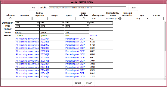
Quick instructions:

• Data is typically rightmost columns. Click to set the top left cell of the data. Columns to the left will be marked as axes.
• Select “axis” in the Dimension dropdown to include a column as an axis. Column data turns blue.
• Select “ignore” in the Dimension dropdown to exclude a column. Column data turns red.
• Select “data” in the Dimension dropdown to treat a column as a data column. Column data turns black.
• Select Type for included axis columns. Select one of three types:

  string

  most general type, data treated as is.

  value

  value data must be numerical and not quoted, e.g. 1, 2

  time

  data must refer to date-time data. Format field may be used to control interpretation of this data. Blank format assumes data contains year/month/day/hour/minute/second separated by some non-numerical character. If fewer than 6 numerical fields present, smallest units are set to minimum value (0 or 1 respectively).

• Click OK button.
• Data is imported into the parameter.
• You may now need to set units for the imported data field, which is located at Edit $\rightarrow$ Dimensions.

In the case shown above, the system has automatically guessed that the data is 3 dimensional, and that the first 3 columns give the axis labels for each dimension (shown in blue), and the 4th column contains the data. The first row has been automatically determined to be the first row of the file -- with the dimension names are shown in green.

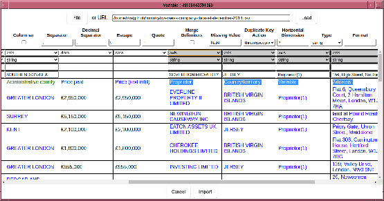
In this case, the automatic parsing system has worked things out correctly, but often times it needs help from the computer user. An example is as follows:

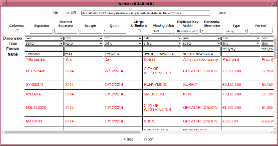
In this example, Minsky has failed to determine where the data starts, probably because of the columns to the right of the “Price” columns. So the first thing to do is tell it where the data is located by clicking on the first cell of the data region.

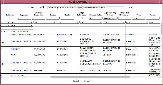
Note that this causes all columns to the right of “Price paid” to be treated as data, which is not right since the columns to the right of “Propieter” are text based columns, not data. So we need to mark those columns as either “axis” or “ignore”. To do that, select drag on the header field, which will cause those columns to be selected, like so:

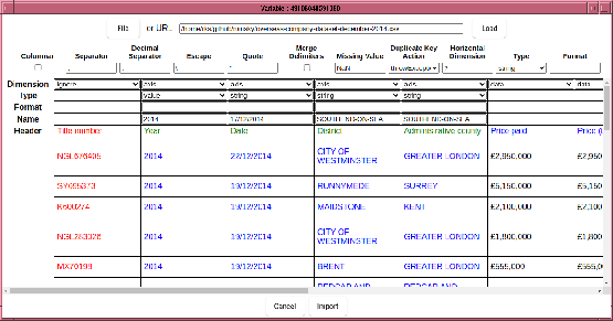
Then in the dimensions row, select “axis”, which flips the selected columns:

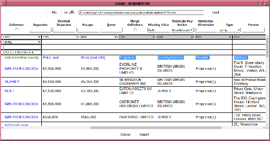
Now the axes index labels are rendered in blue, the axes names in green and the data is in black. In this example, some axes have unique values, which are not particularly useful to scan over. Other examples might have columns that duplicate others, in effect the data is a planar slice through the hypercube. We can remove these axes from the data by marking the column “ignore” in the “Dimension” row. The deselected columns are rendered in red, indicating data that is commented out:

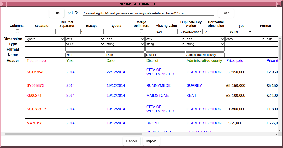
In this example, the axis names has not been correctly inferred. Whilst, one can manually edit the axis names in the “Name” line, a quick shortcut is to drag “Header” and drop it on “Name”. (Note the intention is for this to be the case - currently each column name has to be set individually).

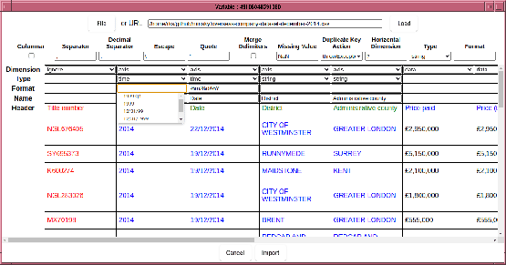
The Date column is current parsed as strings, which not only will be sorted incorrectly, but even if the data were in a YYYYMMDD format which is sorted correctly, will not have a uniform temporal spacing. It is therefore important to parse the Date column as temporal data, which is achieved by changing the column type to “time”, and specifying a format string, which follows strftime conventions with the addition of a quarter specifier (%Q).

If your temporal data is in the form Y*M*D*H*M*S, where * signifies any sequence of non-digit characters, and the year, month, day, hour minutes, second fields are regular integers in that order, then it suffices to use the blank format string . If some of the fields are missing, eg minutes and seconds, then they will be filled in with sensible defaults.

Table 4.1: Table of strftime codes

Code	Description
%a or %A	The name of the day of the week according to the current locale, in abbreviated form or the full name.
%b or %B	The month name according to the current locale, in abbreviated form or the full name.
%d	Day of month in range 01 to 31
%H	Hour in range 0 to 23
%I	Hour in range 1 to 12
%m	Month as a decimal number (01 to 12)
%M	Minute in range 00 to 59
%Q	Quarter (0=1st January, 1=1st March etc)
%p	AM or PM
%s	Number of seconds since epoch (1st January 1970)
%S	Seconds in range 00 to 59
%y	Two digit year YY
%Y	Four digit year YYYY
%z	numerical timezone offset
%Z	Timezone name
%%	Literal % character

Strftime formatted string consists of escape codes (with leading % characters). All other characters are treated as matching literally the characters of the input. So to match a date string of the format YYYY-MM-DD HH:MM:SS+ZZ (ISO format), use a format string “%Y-%m-%d %H:%M:%S+%Z”. Similarly, for quarterly data expressed like 1972-Q1, use “%Y-Q%Q”. Note that only %Y and %y can be mixed with %Q (nothing else makes sense anyway).

Even in the current settings, you may still get a message “exhausted memory -- try reducing the rank”, or a similar message about hitting a 20% of physical memory threshold. In some cases, “titles” and “addresses” might be pretty much unique for each record, leading to a large, but very sparse hypercube. If you remove those columns, then you may encounter the “Duplicate key” message. In this case, we want to aggregate over these records, which we can do by setting “Duplicate Key Action” to sum or maybe average for this example. After some additional playing around with dimensions to aggregate over, we can get the data imported.