Basic System Dynamics model

In 1965, Richard Goodwin, the great pioneer of complexity in economics, presented the paper “A Growth Cycle” to the First World Congress of the Econometric Society in Rome. It was later published in a book collection (Goodwin, Richard M. 1967. "A Growth Cycle," in C. H. Feinstein, Socialism, Capitalism and Economic Growth. Cambridge: Cambridge University Press, pp. 54-58.); to my knowledge it was never published in a journal.

Goodwin's model has been subjected to much critical literature about implying stable cycles, not matching empirical data, etc., but Goodwin himself emphasized that it was a “starkly schematized and hence quite unrealistic model of cycles in growth rates". He argued however that it was a better foundation for a more realistic model than “the more usual treatment of growth theory or of cycle theory, separately or in combination.”

Goodwin emphasized the similarity of this model to the Lokta-Volterra model of interacting predator and prey, which can make it seem as if it was derived by analogy to the biological model. But in fact it can easily be derived from a highly simplified causal chain:

• The level of output ($Y$) determines the level of employment ($L$), with $L=Y/a$ where $a$ is a measure of labor productivity;
• Given a population $N$, the employment rate $\lambda=L/N$ plays a role in determining the rate of change of the wage $w$: Goodwin used a linear approximation to a non-linear “Phillips Curve”:
  

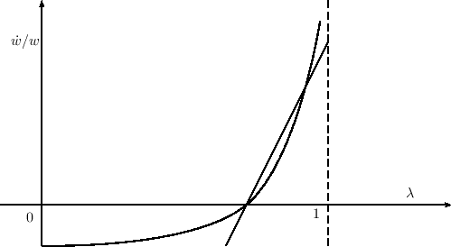
  His linear approximation was:

  
  

  $$\frac1w\frac{d}{dt}w=-\gamma+\rho\cdot\lambda$$
  
  

• In a simple two-class model, profits $\Pi$ equals the level of output $Y$ minus the wage bill: $\Pi=Y-wL$
• For simplicity, Goodwin assumed that all profits were invested, so that Investment equals profits: $I=\Pi$.
• Investment is the rate of change of the capital stock $K$;
• The level of output is, to a first approximation, determined by the level of capital stock ($K$). A simple way of stating this is that $Y$ is proportional to $K$: $Y=K/v$, where $v$ is a constant (Goodwin notes that this relation “could be softened but it would mean a serious complicating of the structure of the model”); and finally
• Goodwin assumed that labor productivity grew at a constant rate $\alpha$, while population grew at a constant rate $\beta$.

  Goodwin published the model as a reduced form equation in the two system states the employment rate ($\lambda$) and the workers' share of output ($\omega$):

  $$\begin{eqnarray*} \frac{d}{dt}\lambda&=&\lambda\left(\frac{1-\omega}{v}-\alpha-\... ...}\omega&=&\omega\cdot\left(\rho\cdot\lambda-\gamma-\alpha\right) \end{eqnarray*}$$
  
  
  
  

This form is useful for analytic reasons, but it obscures the causal chain that actually lies behind the model. With modern system dynamic software, this can be laid out explicitly, and we can also use much more meaningful names. We'll start with defining output (which is a variable). Click on on the Icon Palette, or click on the Operations menu and choose “Variable”. This will open up the “Specify Variable Name” window:

Enter “GDP” into the “Name” field, and leave the other fields blank--since GDP is a variable and we're defining a dynamic system, the value of GDP at any particular point in time will depend on the other entities in the model. Now Click OK (or press “Enter”). The variable will now appear, attached to the cursor. Move to a point near the top of the screen and click, which will place the variable at that location.

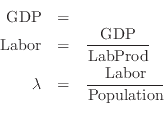
We are now going to write the first part of the model, that Labor (Labor) equals output (GDP) divided by labor productivity (LabProd). Just for the sake of illustration, we'll make a a parameter, which is a named constant (this can easily be modified later). For this we start by clicking on on the Palette, or by choosing Insert/variable from the menu. This will pop-up the Edit Constant window:

There is actually no real difference between the “Edit constant” dialog and the “Edit variable” dialog. The window's title differs, and the default value of Type is “constant” instead of “flow”. We're going to select “parameter”, allowing one to give the parameter a name.

Give the paramter the name “LabProd” and the value of 1 (i.e., one unit of output per worker). Click OK or press Enter and the constant will now be attached to the cursor. Place it below GDP:

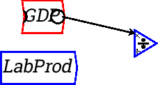
Now we need to divide GDP by LabProd. Click on the symbol on the palette and the symbol will be attached to the cursor. Drag it near the other two objects and click. Your Canvas will now look something like this:

Now to complete the equation, you have to attach GDP to the top of the divide block and LabProd to the bottom.

Now move your cursor to the right hand side of and click, hold the mouse button down, and drag. An arrow will come out from . Drag this arrow to the top of the divide block (where you'll see a tiny multiply sign) and release the mouse. You should then see this:

When the mouse hovers over a block, you will then see little circles that identify the input and output ports of the block:

Those are the connection points for wires, so start dragging from one and release on the other. Now wire LabProd to the bottom of the Divide block (where you'll see a miniature divide symbol (blown up below):

Then click on in the Design Icons to create a new variable, call it Labor, place it the the right of the Divide block, and wire the output port from the Divide block to the input port for Labor:

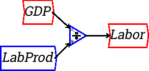
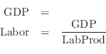
To show the correspondence between the flowchart above and standard modeling equations, click on the equations tab:

$$\begin{eqnarray*} \mathrm{GDP}&=&\\ \mathrm{Labor}&=&\frac{\mathrm{GDP}}{\mathrm{LabProd}}\\ \end{eqnarray*}$$

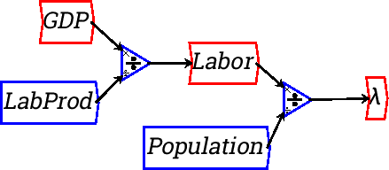
Now let's keep going with the model. With Labor defined, the employment rate will be Labor divided by Population. Define Population as a parameter (we'll later change it to a variable), and give it a value of 110.

Add it to the Canvas and you are now ready to define the employment rate--another variable. Click on , give it the name “$\backslash$lambda” (be sure to include the backslash symbol), put another Divide block on the canvas, choose Wire mode and wire this next part of the model up. You should now have:

Now switch to the equations tab, and you will see

$$\begin{eqnarray*} \mathrm{GDP}&=&\\ \mathrm{Labor}&=&\frac{\mathrm{GDP}}{\mathr... ...rod}}\\ \lambda&=&\frac{\mathrm{Labor}}{\mathrm{Population}}\\ \end{eqnarray*}$$

Notice that Minsky outputs a Greek $\lambda$ in the equation. You can input such characters directly, if your keyboard supports them as unicode characters, however you can also use a subset of the LaTeX language to give your variables more mathematial names.

With the employment rate defined, we are now ready to define a “Phillips Curve” relationship between the level of employment and the rate of change of wages. There was far more to Phillips than this (he actually tried to introduce economists to system dynamics back in the 1950s), and far more to his employment-wage change relation too, and he insisted that the relationship was nonlinear (as in Goodwin's figure above). But again for simplicity we'll define a linear relationship between employment and the rate of change of wages.

Here we need to manipulate the basic linear equation that Goodwin used:

$$\frac1w\frac d{dt}w = -\gamma+\rho\cdot\lambda$$

Firstly multiply both sides by $w$:

$$\frac d{dt}w = w\cdot(-\gamma+\rho\cdot\lambda)$$

Then integrate both sides (because integration is a numerically much more stable process than differentiation, all system dynamics programs use integration rather than differentiation):

$$w=w_0+\int w\cdot(-\gamma+\rho\cdot\lambda)$$

In English, this says that the wage now is the initial wage plus the integral of the wage multiplied by its rate of change function. That's what we now need to add to the Canvas, and the first step is to spell out the wage change function itself. Firstly, since we're using a linear wage response function, the rate of employment has to be referenced to a rate of employment at which the rate of changes is zero. 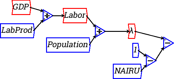I suggest using Milton Friedman's concept of a “Non-Accelerating-Inflation-Rate-of-Unemployment”, or NAIRU. We need to define this constant, subtract it from 1, and subtract the result from the actual employment rate $\lambda$. To enter 1, click on , define a constant and give it a value of 1. Then define another variable NAIRU, and give it a value of 0.05 (5% unemployment). Select “parameter” as the variable type. Subtract this from 1 and subtract the result from $\lambda$. You should have the following:

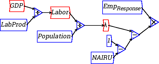
Now we need to multiply this gap between the actual employment rate and the “NAIRE” rate by a parameter that represents the response of wages to this gap. Let's call this parameter Emp_{Response} (remember to include the underscore and the braces). Define the parameter, give it a value of 10, and multiply ($\lambda$ minus NAIRE) by it:

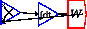
Now we are ready to add a crucial component of a dynamic model: the integral block, which takes a flow as its input and has the integral of that flow as the output. The wage rate w is such a variable, and we define it by clicking on the symbol in the Icon Palette (or by choosing Operations/Integrate from the Insert menu). This then attaches the following block to the cursor:

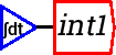
Now we need to rename this from the default name of “int1” to “w” for the wage rate. Either right click or double-click on “int1” and this will bring up the edit window . Rename it to “w” and give it a value of 1:

To compete the integral equation, we need to multiply the linear employment response function by the current wage before we integrate it (see the last equation above). There are two ways to do this. First, place a multiply block between the wage change function and the integral block, wire the function up to one input on the multiply block, and then either:

• wire the output of the w block back to the other input on multiply block; or
• Right-click on w, choose “Copy Var”, place that copy before the multiply block, and wire it up.

The first method gives you this initial result:

That looks messy, but notice the blue dot on the wire? Click and drag on that and you will turn the straight line connector into a curve:

The second approach, which I personally prefer (it's neater, and it precisely emulates the integral equation), yields this result:

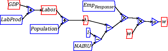
From this point on the model develops easily--“like money for old rope”, as one of my maths lecturers used to say. Firstly if we multiply the wage rate w by Labor we get the Wage Bill. To do this, firstly create the variable Wage Bill, and put it well below where $w$ currently is on your diagram:

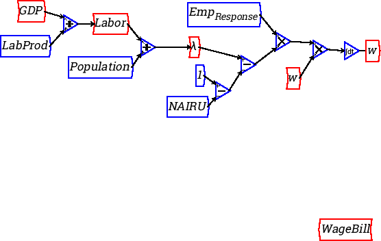
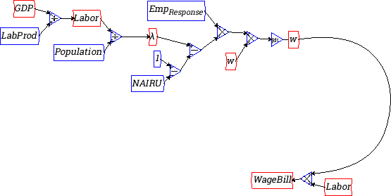
Now right-click on WageBill and choose “Flip”. This rotates the block through 180 degrees (any arbitrary rotation can be applied from the variable definition window itself). Now right-click on Labor, which you've already defined some time ago, and choose “Copy”. Place the copy of Labor to the right of WageBill:

Now insert a multiply block before WageBill, and wire w and Labor up to it. Curve the wire from $w$ using the blue dots (you can do this multiple times to create a very curved path: each time you create a curve, another 2 curve points are added that you can also manipulate, as I have done below:

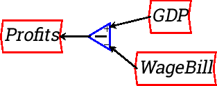
The next step is to subtract the WageBill from GDP to define Profits. Take a copy of GDP, insert it above WageBill, insert a subtract block, and wire it up to define the variable Profits:

In the simple Goodwin model, all Profits are invested, and investment of course is the rate of change of the capital stock Capital. Create a variable called Investment, wire this up to Profits, and then create a new integral variable Capital using the icon. Right-click or double-click on it to rename int2 to Capital, and give it an initial value of 300:

Wire this up to Investment:

Now there's only one step left to complete the model: define a parameter CapOutputRatio and give it a value of 3:

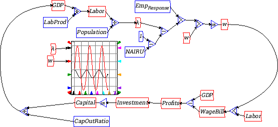
Divide Capital by this, and wire the result up to the input on GDP. You have now built your first dynamic model in Minsky:

Before you attempt to run it, do two things. Firstly from the Runge Kutta menu item, change the Max Step Size to 0.01--to get a smoother simulation.

Secondly, add some graphs by clicking on the icon, placing the graph in the middle of the flowchart, and wiring up $\lambda$ and $w$ to two of the four inputs on the left hand side. You will now see that, rather than reaching equilibrium, the model cycles constantly:

If you click on the equations tab, you will see that you have defined the following system of equations:

$$\begin{eqnarray*} \mathrm{GDP}&=&\frac{\mathrm{Capital}}{\mathrm{CapOutRatio}}\\... ...times w\\ \frac{d\mathrm{Capital}}{dt}&=&\mathrm{Investment}\\ \end{eqnarray*}$$

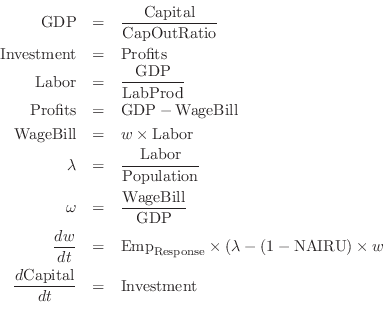
At this level of complexity, the equation form--if you're accustomed to working in equations--is as accessible as the block diagram model from which it was generated. But at much higher levels of complexity, the block diagram is far easier to understand since it displays the causal links in the model clearly, and can be structured in sub-groups that focus on particular parts of the system.